Audio 101: Issue Three

Hello! It's been too long since issue two, so let's jump straight into it. The lossless file you're listening to might actually be a lossy file in disguise (Juice WRLD's entire catalogue is lossy!). The remaster you're listening to is probably worse than the original too.

Today we'll learn about spectrograms and waveforms. By the end of this thread, you'll be able to read both these graphs. You'll be able to identify bad masters and differentiate lossy audio from lossless audio. Strap in, this issue is very dense.

Waveforms represent loudness over time. x-axis is time, y-axis is loudness. Longer the lines, louder the volume. It's very useful for analysing dynamic range and clipping. Top one is left channel, bottom is right. I'm using Audacity for these waveforms.

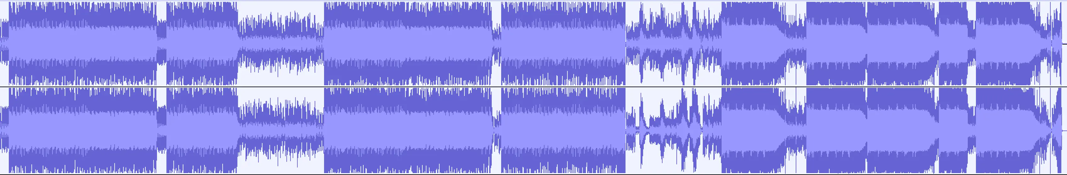
If you’re trying to compare dynamic range, I recommend normalizing both tracks to the same volume (I use -14 LUFS). You can do this in Audacity with Effect -> Volume and Compression -> Loudness Normalization.

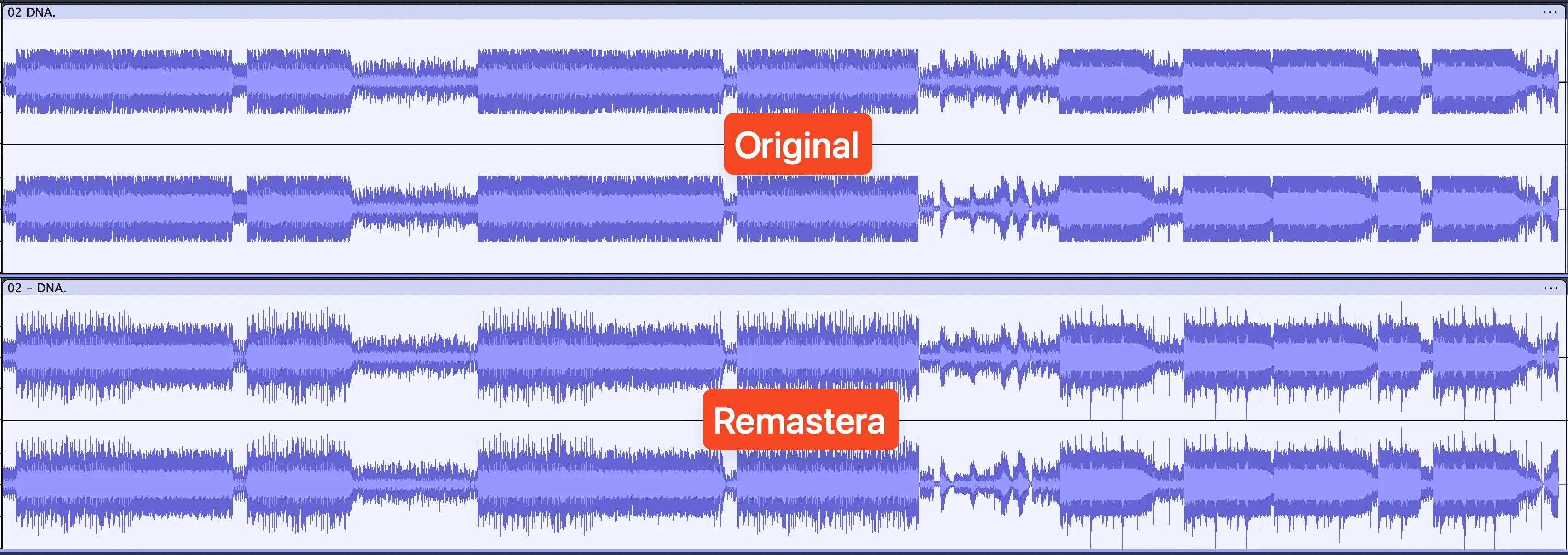
Notice how the lines in the Remastera version are far more dynamic. You can see a sharp cutoff in the original, this is an indicator of heavy compressors and limiters. The chunkier it looks, the stuffier it sounds.

I also suggest turning on "Show Clipping in Waveform" option in Audacity's View menu, it'll show clips as red lines. When the line exceeds the boundaries (i.e. it's too loud) it becomes noise. This is called clipping.

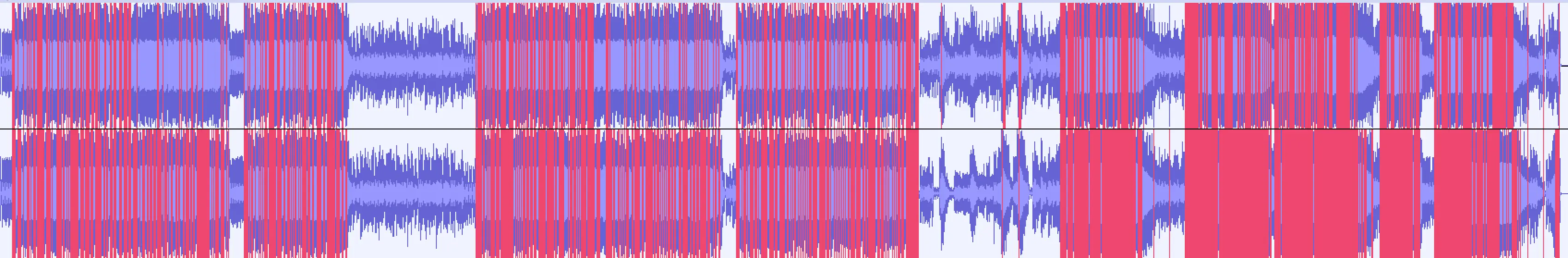
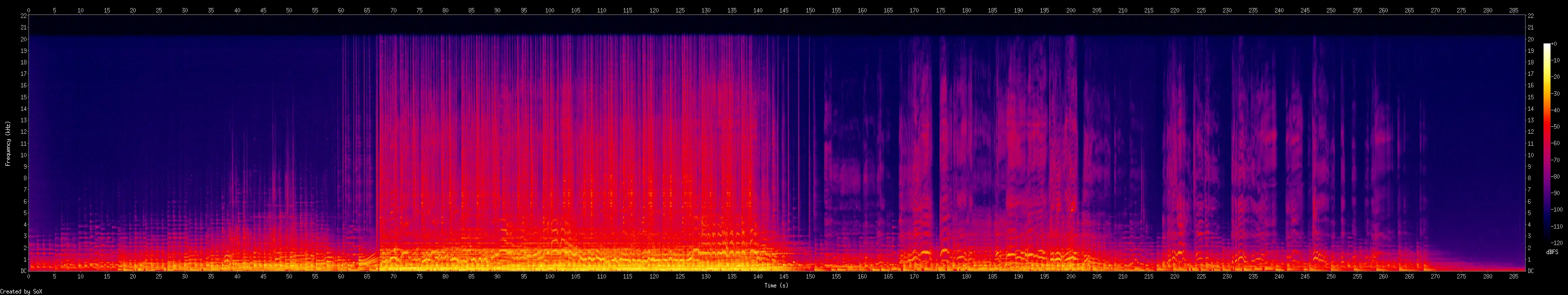
You can use waveforms to compare originals to their remasters. Once you start doing this, you’ll realize how bad remasters are - ruined dynamic range and clips everywhere. If the original is bad, like in the showcased example, Remastera has your back.

Spectrograms add one more data point to this graph. It not only shows loudness over time, it shows which frequency is loud when. It has three axes: x-axis is time, y-axis is frequency, z-axis is the colour itself. Brighter the colour, louder the sound.

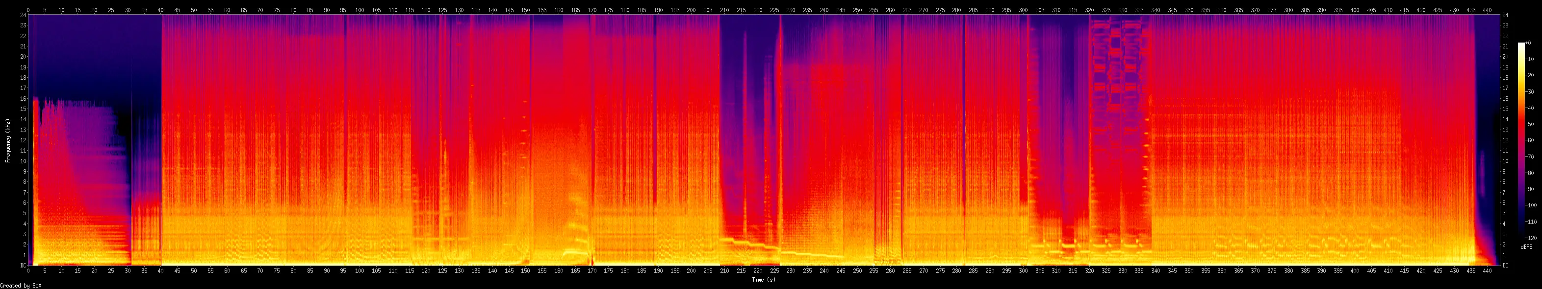
I use Sox to generate spectrals. The commands I use:

Full length:

sox input.flac -n remix 1 spectrogram -x 3000 -y 513 -z 120 -w Kaiser -o spectral.png

Specific timeframe (2 seconds from 0:30):

sox input.flac -n remix 1 spectrogram -X 500 -y 1025 -z 120 -w Kaiser -S 0:30 -d 0:02 -o spectral_zoomed.png

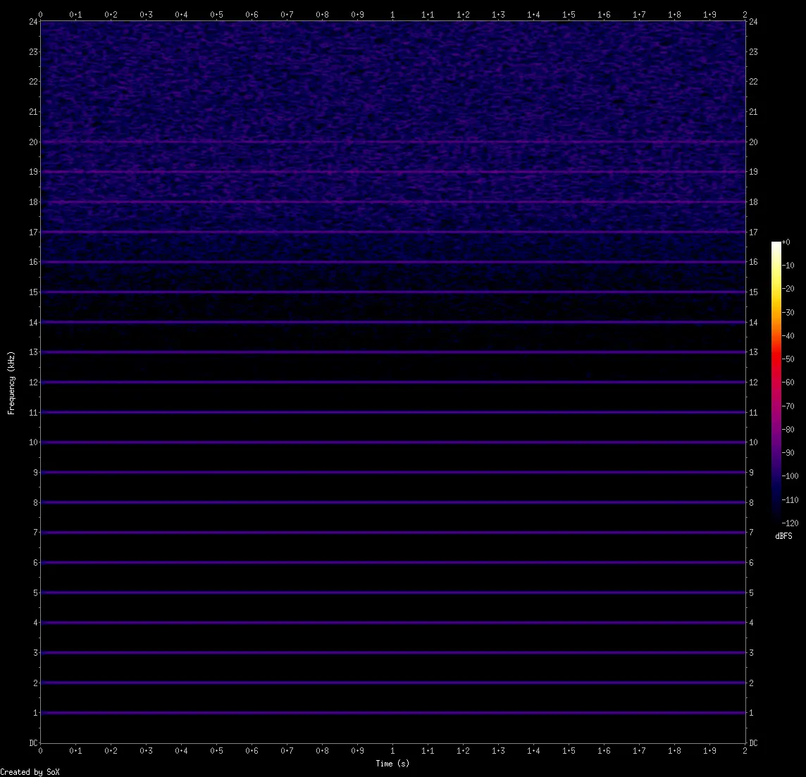
Look at this simple spectrogram. The audio is a simple sine wave (-90 dBFS) recurring every 1 kHz. With a waveform, we wouldn't be able to tell the frequencies at which the sine waves occur.

Info dump time. Artists don’t always put out their tracks in lossless formats. I’m not talking about recording equipment or dithering algorithms. They straight up export in MP3 and release it sometimes. We call these lossy masters. Juice WRLD is a famous example.

When you download a lossless audio file, you can never be sure it's actually lossless. It might actually be MP3s or other lossy codecs converted to a FLAC/WAV file. They're more common than you think.

What's worse is a lossy file converted to another lossy file. YouTube MP3 downloaders for example. YouTube doesn't provide MP3 files, it's almost always Opus - a lossy codec. These websites convert Opus to MP3 (lossy to lossy conversion), causing much greater data loss.

With spectral analysis, you’ll be able to identify these files. Lossy masters, fake lossless files and lossy to lossy encodes. There's a reason this hasn't been automated - it can get very tricky. I'll explain the basics here.

In the previous issue, I went into detail on how our hearing drops rapidly above 16 kHz, and how lossy codecs take advantage of this. The following two characteristics are direct results of that fact. Let's get back to the pretty images!

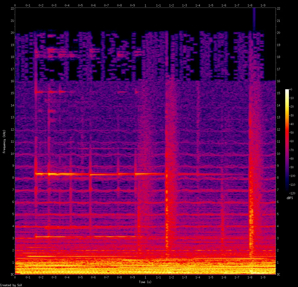
Lowpass filters are cutoffs in the spectral, typically between 16-20 kHz. Cutoffs don't automatically imply that the file is lossy, though. This spectral is Great Gig In The Sky by Pink Floyd (1983 CD). It has a cutoff at 20 kHz, but it's not been through a lossy encoder.

So this doesn't mean that files that have no data above a certain frequency range are lossy. Classical music has almost no data beyond 10 kHz. It's highly dependent on the genre and instruments.

Shelves are like cutoffs but not as abrupt. This is a V0 MP3 of the lossless file shown above.

Blocks (or clumps) are more subtle but if you find them, it's a guarantee that the file has been through a lossy encoder. Only lossy encoders make these blocks (but not all lossy encoders do). If only few regions contain blocks, those particular samples are lossy.

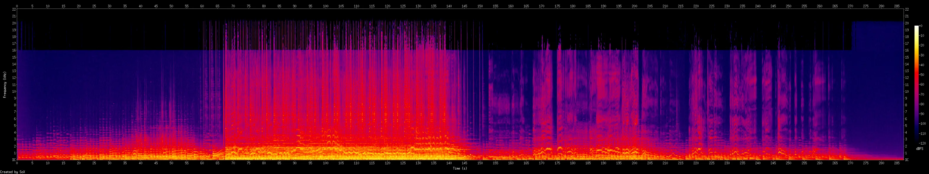
Here's an example containing all the above. Cutoff at 20 kHz, shelf at 16 kHz, with blocks (those rectangular clumps) above the shelf. This is a 320kbps MP3.

Identifying lossy to lossy encodes is... complicated. If you find signs of MP3 cutoffs or shelves in a, say, Opus file, it's highly likely that the Opus was made from MP3. Or if you find cutoff patterns of 192kbps MP3 in a 320kbps MP3 file.

Other than specific cases like these, it's nearly impossible. Modern codecs are getting so good, it's hard to tell. There are patterns though. I can’t list them all here, but you will find them as you deal with spectrals more.

For example, Opus files are always 24 kHz and they have noise-shaped dither reaching all the way to 14 kHz. These combined are dead giveaways. Every codec will have a weakness. A characteristic. The more you deal with them, the better you get at identifying them.

That’s it for this issue. It’s been four months since the last one! My bad. As always, if you have any questions, feel free to reply. Until next time. Cheers!